Python Skills
This section of my portfolio was created during a class I took in graduate school. The class is the following:
GEOG 4092 - GIS Programming and Automation (3 Credits): Students will learn the most commonly used programming language to automate GIS geoprocessing tasks and workflows in the latest versions of the most popular GIS systems.
Below are the labs conducted in that class. They start simple and get increasingly hard.
Lab 0
For and While Loops
Goal: Learn the basics of Python. Gain an introductory understanding of common Python objects and basic operators and structures. Become familiar with the JupyterLab platform.
-
Create a list of hypothetical file names using a for loop: a) Create a list with the following strings as elements: 'roads', 'cities', 'counties', 'states' b) Create an empty list and then populate it by concatenating each of the strings above with ‘.txt’. This should result in a list of strings ending in .txt (e.g. ‘roads.txt’, ‘cities.txt’, etc.).
-
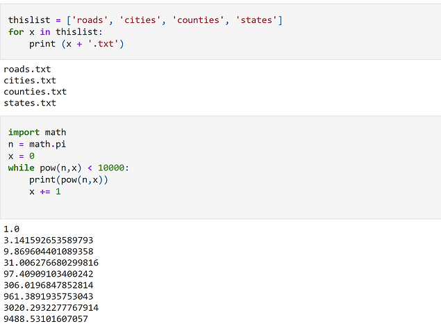
Write a while loop that raises the mathematical constant pi (3.14159…) to its powers until the result is greater than 10,000 (i.e. pi0 , pi1 , pi2 ,…). HINT: You will need to import the math module. Examine the while loop examples in code_examples/python_basics.py (on Canvas) to figure out how to set up the loop structure. What condition are you testing
Lab 1
Data Preparation and Vector Geoprocessing
Goal: Learn to work with multiple data files in an automated framework. Gain familiarity with the Pandas and Geopandas module to conduct vector geoprocessing and relational joins.
Data: Download the file lab1.zip from Canvas and unzip it into your home directory. The geopackage (lab1.gpkg) contains a feature class of two watersheds in northern Colorado and spatial and tabular data from the USDA Soil Survey Geographic Database (SSURGO). There are 9 feature classes that cover the area of the two watersheds. The feature classes delineate survey polygons used to record soil properties in SSURGO. The file geodatabase also contains 9 tables with attribute data that correspond to the feature classes. Column names in the tables correspond to the following: musym (map unit symbol, which is a classification scheme for mapped areas); aws025wta (available water storage 0-25cm); aws0150wta (available water storage 0-150cm); and drclassdcd (drainage class, indicating the dominant condition).
Task: You will process the SSURGO data by joining each of the tables to the corresponding feature class and then you will merge the 9 feature classes. Next, you will intersect the SSURGO data with the watershed boundaries and finally count the number of map unit polygons within each watershed.
Part I:
-
Join each of the tables to the corresponding feature class. Find a common field to join on.
-
Add a new field named mapunit to each joined feature class and calculate the values for all features as the map unit ID of the feature class. The map unit ID is the suffix of the layer name (e.g., co641).
-
Merge the 9 feature classes into a new feature class.
-
Intersect the merged feature class with the watershed boundaries.
Part II:
Find the number of features in the resulting intersected feature class that correspond to each watershed. Report these two numbers in a print statement at the end of your script. Hint: Look at the groupby function from pandas, which column should you group by

Lab 2
Vector Encoding
Goal: Learn to encode vector geometry. Gain familiarity with Shapely, and Geopandas properties.
Data: Download the file lab2.zip from Canvas and unzip it into your home directory. The data folder contains three text files and two geotiff raster files. The text files contain coordinates delineating the boundaries of three districts (administrative units) in eastern Tanzania. The rasters are from the 2004 and 2009 GlobCover dataset, which is a global land cover classification with a nominal spatial resolution of 300 meters. The GlobCover layers have been reclassified to look solely at agricultural lands. Each is a Boolean raster where 1 represents land utilized for agriculture and 0 represents all other land cover classes. Task: You will encode the text files into polygon features. Then you will calculate percentage of agricultural land in each polygon in 2004 and in 2009 using the GlobCover rasters.
Part I:
-
Read the text files and extract the x, y coordinates for each district.
-
Create a polygon from each file and create a geodataframe with the following two fields: ‘num_coords’ and ‘district’. populate the corresponding value for the two fields you added. ‘num_coords’ should contain the number of vertices, or coordinate pairs, used to encode each polygon. ‘districts’ should be the suffix of each text file (i.e., ‘01’, ‘05’ or ‘06’). Hint: steps 1 and 2 should be done concurrently as you encode the polygons. TIP: What are the methods to create a geodataframe? Which data structure allows for data schema (pre-defined data structure such as column names)
Part II:
-
Calculate the number of agricultural pixels in each district (i.e., each polygon) in 2004 and in 2009.
-
In a final print statement, report the amount of agricultural land as a percentage of the total number of pixels in each district in 2004 and in 2009 (i.e., print these six values)

Lab 3
Random Spatial Sampling
Objective: Learn about spatial sampling, particularly random sampling regimes. Broaden understanding of vector geometry structures to encode and deconstruct objects. Learn to effectively implement functions in your code.
Data: Copy the lab3.zip file from Canvas into your working directory. This lab will use the SSURGO data from lab1, but for larger extent, and watersheds for the same area at two different levels of detail (HUC8 and HUC12). The HUC classification is a hierarchical system, where level 12 watersheds are nested within larger level 8 watersheds. We will use the available water storage 0-150cm (aws0150) variable from the SSURGO data in this lab.
Goals: Write a generic framework that implements a stratified random sampling of points within a polygon feature class. Generate two stratified random samples based on point density within the HUC8 and HUC12 watersheds. Then summarize the aws0150 variable based on each sample. Compare the mean values of aws0150 within each HUC8 watershed based on the two sampling routines conducted within the HUC8 versus the HUC12 boundaries.
Part I: Create a stratified random sampling approach for HUC8 and HUC12 watersheds
A. Calculate the number of points (n) to sample in each polygon (i.e., watershed).
-
Get the extent of the polygon.
-
Get the area of the polygon, and convert it to square kilometers.
-
Calculate the number of points using a point density of 0.05 points/sqkm. Round to the nearest integer.
B. Create a stratified random sample of n points within each polygon.
-
Randomly generate points within the extent of the polygon using random seed 0, i.e., random.seed(0).
-
Test if each point is within the polygon boundary.
-
If so, encode the point and indicate the HUC8 watershed that contains the point.
Part II: Summarize the SSURGO attributes by level of sampling
-
Calculate the mean aws0150 for each HUC8 watershed from the HUC8- and HUC12-based point samples, i.e., you will have three mean values for each point sample. Hint: look at the pandas group by method.
-
In a final print statement, report the mean values for each HUC8 watershed from the two samples and your conclusions regarding the different results of sampling within HUC8 versus HUC12 watersheds. You should print out six total mean values (three for the HUC8-based point sample and three for the HUC12-based sample.
-
Implement at least one meaningfully used function. This means that your function effectively creates a useful, reusable operation. Functions should be put at the top of your script and should be well documented.

Lab 4
Raster convolution with NumPy
Scenario: You have been contracted to conduct a site suitability analysis for a wind farm in the Philippines. Based on wind resource data and a set of exclusions, you will identify potential sites for the wind farm. You will then calculate the distance from potential sites to electricity grid transmission substations.
Data: Copy the lab4.zip file from Canvas into your working directory. The data folder includes five raster layers: urban areas (urban_areas.tif), water bodies (water_bodies.tif), IUCN-1b protected areas (protected_areas.tif), slope in degrees (slope.tif), and mean annual wind speed in meters per second (m/s) at 80m hub height (ws80m.tif). All layers are in the same projected coordinate system with the same spatial resolution. There is also a text file with the coordinates for grid transmission substations.
Overview: You will create a final suitability surface of potential sites for the wind farm by combining the raster layers. To do so, you need to create Boolean arrays for the five different selection criteria based on the thresholds specified below. You will develop a framework for conducting moving window operations. The dimensions of the moving window will be 11km North-South by 9km East-West, producing 99km2 potential wind farm sites. Finally, you will calculate the Euclidean distance between the center of suitable sites and the closest transmission substation.
Selection Criteria: The following five conditions for the potential sites are the basis for your suitability analysis:
-
The site cannot contain urban areas.
-
Less than 2% of land can be covered by water bodies.
-
Less than 5% of the site can be within protected areas.
-
An average slope of less than 15 degrees is necessary for the development plans.
-
The average wind speed must be greater than 8.5m/s.
Part I: Evaluate site suitability
-
Write a generic framework for calculating the mean value of a raster within a moving window, i.e., create a focal filter using NumPy:
-
Create an empty output array to store the mean values.
-
Loop over each pixel (each row and column) and calculate the mean within the moving window. The window dimensions must be 11 rows by 9 columns. Ignore the edge effect pixels.
-
Assign the mean value to the center pixel of the moving window in the output array.
-
-
Evaluate each of the selection criteria to produce five separate Boolean arrays.
-
Create a surface of suitability values by summing the five Boolean arrays. Only sites with a score of 5 will be considered; create a final Boolean suitability array indicating the location of the selected sites.
-
Convert your final numpy suitability array to a geotif raster file for visualization purposes. 5. In a final print statement, report the number of locations you found with a score of five.
Part II: Calculate distance to transmission substations and implement functions
-
Using the substation coordinates, calculate the Euclidean distance from the centroid of each suitable site (i.e., with a score of 5) to the closest transmission substation. Print the shortest and longest distance to the closest transmission substation among all of the suitable sites, i.e., you will only print two distances.
-
Effectively implement functions for reusability and overall organization

Lab 5
Vegetation Recovery after Wildfire
Scenario: You have been contracted by the U.S. Forest Service to model vegetation recovery after the Big Elk wildfire, which burned 4,413 acres between Lyons and Estes Park in July 2002. Your task is to analyze the relationship between recovery and terrain, specifically slope and aspect. As an independent contractor with a small budget you do not have access to an ArcGIS license, so you will have to conduct the analysis with open source tools.
Data: Extract the lab5.zip file from Canvas into your working directory. The data folder contains the following: a subfolder named L5_big_elk, which contains bands 3 and 4 (the red and near infrared bands, respectively) for a series of Landsat 5 Thematic Mapper (TM) images from 2002 to 2011 (all images were captured between August and October); a raster delineating the fire perimeter and an area of healthy forest outside of the fire perimeter (values of 2 indicate healthy forest, values of 1 indicate burned pixels, and values of 255 indicate a transition zone between the two that will be excluded from the analysis); and a DEM.
Goal: You will use the open source module Rasterio for input/output (I/O) to work with spatial data in Python. Building on your experience of Numpy and Scipy, you will use these tools for spatiotemporal raster analysis. You will work with some helper functions that I have prepared for you and build on these tools to develop your own open source solutions. You will write your own zonal statistics function in this lab and learn to use the Pandas module.
Overview: The Normalized Difference Vegetation Index (NDVI) can be used to measure relative abundance of green vegetation and biomass production. NDVI is calculated from the red and near infrared bands of a remotely sensed image. Environmental conditions change from year to year and season to season. So, comparing biomass production and abundance between two points in time with satellite imagery comes with a significant amount of uncertainty. Variation in atmospheric conditions, scene illumination and sensor viewing geometry further complicate temporal comparison. In light of this, you will calculate a Recovery Ratio (RR) between the NDVI of each burned pixel inside the fire perimeter and the mean NDVI of healthy forest pixels outside of the burned area. This allows you to estimate vegetation recovery after the fire while minimizing the aforementioned issue of simply comparing NDVI across the years of analysis. Once you have calculated the RR for each pixel inside the fire perimeter, you will calculate the coefficient of recovery of the RR for each pixel across the years of analysis by fitting a first-degree polynomial. You will then summarize the vegetation recovery by terrain slope and aspect using a Zonal Statistics operation.
Part I:
-
Read the DEM in as a numpy array and, using the functions provided, calculate the slope and aspect. Reclassify the aspect grid to 8 cardinal directions (N, NE, E, SE, etc.). Reclassify the slope grid into 10 classes using the function provided.
-
Calculate the Normalized Difference Vegetation Index (NDVI) for all years of analysis from the Landsat images.
-
Calculate the Recovery Ratio for each pixel for each year: mean(NDVI of healthy forest). Remember that the denominator is the mean NDVI of all healthy forest pixels for a given year (i.e. for each pixel in a given year, you will use the same number in the denominator). HINT: you can get the denominator using Boolean indexing to subset the values you need.
-
Calculate the trend of the RR for each pixel across the years of analysis.
-
Print the mean RR for each year and also print the mean coefficient of recovery across all years for the burned area (remember, you need to exclude the values outside of the burned area in these calculations).
Part II:
-
Write a generic function that calculates “Zonal Statistics as Table” using two numpy arrays (the zone raster and the value raster). Your function should calculate: mean, standard deviation, min max and count. Use Pandas to create a dataframe with the zonal output and write the results to a csv file. The zonal output csv file should have the zone field (slope or aspect classes) and the five statistics (min, max, mean, stddev, and count). Your output csv table should have as many rows as there are unique zone values.
-
Calculate zonal stats of the coefficient of recovery for each terrain slope class and then for each cardinal direction of aspect, which you reclassified in Part I. You should produce two output csv files, one for slope and one for aspect. Since you are only interested in the burned pixels, your zonal stats function must somehow exclude all pixels outside of the fire perimeter. Hint: numpy.nan.
-
Export the final coefficient of recovery np array for the burned area as a GeoTiff (the extent should match that of the inputs). Non-burned pixels should have a NoData value (e.g. -99).
-
What are your conclusions regarding vegetation recovery and terrain? Provide a print statement explaining the relationship you found between slope and aspect of the terrain and vegetation recovery after wildfire